Forecasting Lakers Wins/Losses with Machine Learning and Linear Discriminant Analysis
2023-08-19
| Brief History
I got the idea to do this project from a previous project I did in my STAT 632 class. In that presentation I tried to model the relationship between Points Per Game and several other predictors.
| Context
- Specifically it is the Lakers’ average game data for the 2019-2020 regular season. I was interested in doing this analysis because that season was interrupted by the COVID-19 pandemic, leading the regular season for all teams to end at 73 games instead of the typical 82 game season.
| Context
- At the time of the pandemic, the Lakers had only played 63 games as did other teams, and when it resumed they played an additional 10 games, not including a truncated playoffs. I was interested to see if there would be any differences between the pandemic games versus if the pandemic never happened.
Hypothesis
So, to do this I am interested in forecasting Wins and Losses based on four predictors: Team points, Opponent Points, and Games played with W/L as the response variable.
| Methods: Exploratory Analysis
To start, I did a brief exploratory analysis in R.

Fig 1. Plot of Games versus Team points and Opponent points. Most of the blue curve (Lakers score) was higher than the yellow curve (opponents’ score).
| Analysis
Here is the head of the dataset.
| Games | Team Score | Opponent Score | Wins/Losses |
|---|---|---|---|
| 1 | 102 | 112 | L |
| 2 | 95 | 86 | W |
| 3 | 120 | 101 | W |
| 4 | 120 | 91 | W |
| 5 | 102 | 112 | L |
| Analysis
I performed an 80/20 test and training set split for the data.
| Analysis
I decided to test four different models to see which one was most accurate for my purposes. The dotplot showed that LDA (linear discriminant analysis) would be the best data to help predict W/L.
| Analysis
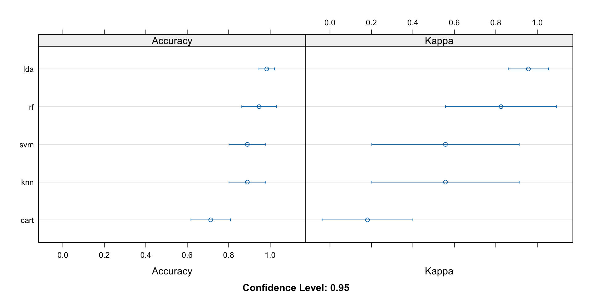
Fig 2. Analysis of the most effective model.
| Analysis
- The next step was to obtain a formula for the linear discriminant which would allow us to assign an LDA score to help us create an LDA score for W/L. The equation for the linear discriminant involving the predictors was
\[ LD1=-0.033G + 1.4956Tm + -1.431Opp \].
| Analysis
- LD scores were calculated for each value and then subtracted from the mean of each LD1 value for those values of LD1 that were a Win for the Lakers, and a Loss. Then those values were averaged to get a LDA score of -0.8667901 or roughly -0.867.
| Analysis: Decision Boundary and LDA Score
- A score of about -0.867 means that, when incorporating other predictors in the LD1 calculation:
- Any value above -0.867 was very likely to be a “W”
- Any value below -0.867 was very likely to be a “L”
| Analysis
Since I already know the numbers of the missing games, the next step was to obtain a Team score and Opponent score based on the data.
- I created a for-loop using an empty data frame to simulate 19 pairs of numbers randomly picked from the uniform distribution, with a min of 84 and a max of 143.
| Analysis
- These min/max numbers are based on the fact that the Lakers lowest/highest score from any game was about an 88 and 142, while the lowest/highest score an opponent ever achieved against the Lakers was about 80 and 139, respectively.
| Analysis
Here are the top 5 data for the predicted scores and W/L.
| G | Predicted Team Score | Predicted Opponent Score | Predicted W/L |
|---|---|---|---|
| 64 | 109 | 134 | W |
| 65 | 93 | 102 | L |
| 66 | 119 | 97 | L |
| 67 | 97 | 114 | W |
Results
From the simulation, I was able to conclude that had the Lakers played all 82 games, they would have won 55 games, and lost 27, with a final win percentage of 67% and a loss percentage of 33%.
- This is lower than what they actually achieved during the truncated regular season, which was 49 W (78%) and 14 L (22.2%) out of 73.